
User-User Collaborative Filtering
Published:
Collaborative filtering is considered to be the most popular and widely implemented technique in Recommender Systems.
Here we implement a User-User Collaborative Filtering model for movie recommendation using the MovieLens dataset on Kaggle. Note that you need to put the original data of the ratings, named rating.csv and save it to the directory Data.
Here we briefly talk about the code and results, and then dive a little bit into the theory of the User-User Collaborative filtering models.
Codes & Results
The code consist of two parts. One is for the data preprocessing, and one implements and tests the User-User Collaborative Filtering.
- The data preprocessing code: It has two main jobs:
- it decreases the size of the data: The original data contains the records for 20 million ratings, which requires a lot of computations. This is specially problomatic if we do not use parallel computations. To allow us to run this code on a pc, we shrink the data to contain only those users that are the among the most common users. Similarly, we filter the data to include only the most common movies. The filtered version of the data, titled small_rating.csv is then saved to the directory Data.
- It extracts the useful information from the small_rating.csv and save it in some dictionaries in the directory Data. We are going to use these dictionaries to implement the User-User collaborative filtering.
- The User-User Collaborative Filtering: This file implements the User-User Collaborative Filtering.
We use 80% of the data (i.e. small_rating.csv) for training and the remaining for the testing. The MSE errors for the training and testing are as follows:
MSE for train set = 0.506464060842711
MSE for test set = 0.6078670855080118
Note that to get a sense of whether this is a good performance or not we need to compare it with a benchmark, which I do not get into the details in here, but one simple case can be to for each user output his/her average rating as the prediction for a new movie. Another important factor is to note that this MSE is for a subset of the data that has most common users and most common movies. If we performe this algorithm on the original data (20 million ratings), it would take considerably longer time to finish the computations, and the error would increase as well for both the train and test set.
Theory of User-User Collaborative Filtering
Here the goal is to design a model that predicts the ratings that a user is going to give to an item that he/she has not rated before (i.e. unseen product). This is practically a regression problem, and the approach we are taking here, i.e. user-user collaborative filtering is basically building a regression model with few extra steps.
The algorithm for the user-user collaborative filtering is summarized in the following:
# User-User Collaborative Filtering
# for predicting the rating that user u gives to item i:
#-------------------------------------------------------
1. For each user v != u:
	   If they have minimum number of common items:
		    Calculate the Similarity Weight between user v and user u
2. Keep only the top neighboring users (There are different techniques for doing this)
3. Calculate the linear average of the normalized ratings that the rop users gave to the item i, and the weights of this linear function are the similarity weights. We also add back the off-set term of the normalization for user u back to the rating.
Note that if we have N users and M movies, when training, we need to: for each user, look at all other users, and, calculate the similarity between the two users (i.e. its a mathematical operation which includes vectors of length #movies). Hence the computational time of this algorithm during the training process is $O(M×N^2 )$, which is considerably high because we usually have a lot more users than movies, i.e. $N \gg M$. Hence later on we will take a look at a modified version of this algorithm called Item-Item Collaborative Filtering, which has a running time of $O(N×M^2)$, which is preferable.
Another common problem is that there may be differences in the users’ individual rating scales. In other words, different users may use different rating values to quantify the same level of appreciation for an item. For example, one user may give the highest rating value to only a few outstanding items, while a less difficult one may give this value to most of the items he likes.
To solve this problem, we normalize the rating by centering them (i.e. subtracting the average ratings that a use gives). This technique is called mean-centering.
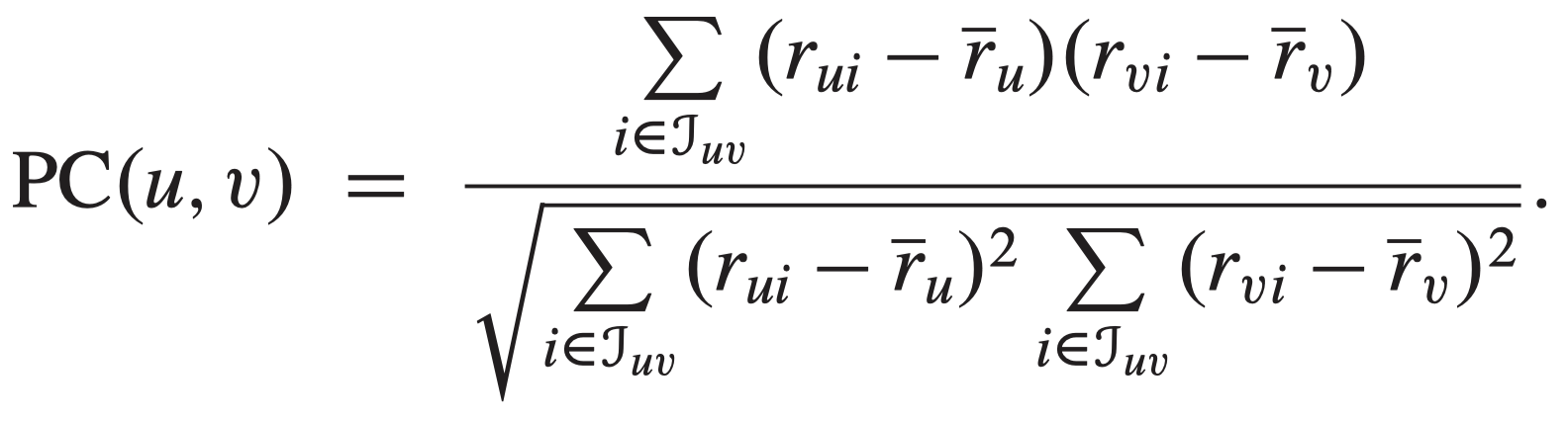
Similarity-Weight:
The choice of the similarity weight is one of the most critical aspects of building a neighborhood-based recommender system. Here we use the Pearson Correlation (PC) similarity metric. It has the effect of normilizing the ratings as the effects of mean and variance have been removed, and the ratings are mean-centered. However, when making a prediction for user u, we need to add the average rating of the user u back to the forecasted rating!
We note that other similarity metrics such as Cosine Ssimilarity, Mean Squared Difference and Spearman Rank Correlation Coefficient. For more info, see Chapter 2 of [1] and [2].
Neighborhood Selection
In general, a small number of high-confidence neighbors is by far preferable to a large number of neighbors for which the similarity weights are not trustable. That is why we are limiting the number of the top neighbors for which we compute the weights for. This also helps the trarining and when performing in real time.
Neighborhood selection happens in two places (we implement this in the code as well):
Pre-filtering of Neighbors
The prefiltering of neighbors is an essential step that makes neighborhood-based approaches practicable by reducing the amount of similarity weights to store, and limiting the number of candidate neighbors to consider in the predictions. Basically, when we are learning the weights for a given user u, we only calculate/store the weights for those who users that (implicitely) are similar enough such that it worth it to perform the computations. There are different approaches to do this:
- Top-N filtering: For each user or item, only a list of the N nearest-neighbors and their respective similarity weight is kept.
- Threshold filtering: Instead of keeping a fixed number of nearest-neighbors, this approach keeps all the neighbors whose similarity weight’s magnitude is greater than a given threshold.
- Negative filtering: In general, negative rating correlations are less reliable than positive ones. We can filter those.
Neighbors in the Predictions
Once a list of candidate neighbors has been computed for each user or item, the prediction of new ratings is normally made with the k-nearest-neighbors, that is, the k neighbors whose similarity weight has the greatest magnitude. The choice of k can also have a significant impact on the accuracy and performance of the system. Note that typically the prediction accuracy observed for increasing values of k follows a concave function. Thus, when the number of neighbors is restricted by using a small k (e.g., k < 20), the prediction accuracy is normally low. As k increases, more neighbors contribute to the prediction and the variance introduced by individual neighbors is averaged out. As a result, the prediction accuracy improves. Finally, the accuracy usually drops when too many neighbors are used in the prediction (e.g., k > 50), due to the fact that the few strong local relations are “diluted” by the many weak ones. Although a number of neighbors between 20 to 50 is most often described in the literature, the optimal value of k should be determined by cross-validation.
To see the Github repository for this project, see Github.