
Finding Control Policy for Mountain Car using TD(λ) and elibility traces for finding the Q-value Function Approximator
Published:
When updating the Q-values (i.e. state-action value functions), the updates coming from the TD(λ) algorithm are given as some mixture of the multi-step return predictions, ranging from TD(0) (which is the original temporal-difference, TD(0), algorithm) to TD(∞) (which is practically speaking the Monte-Carlo approach, and ∞ means “till the end of the episode”).
Now, one can easily see that if we implement TD(λ) without any smart idea, then the computational time would be significant. That smart idea is called eligibility traces which allow the algorithm to be incremental. This idea is also referred to as the Backward-View.
In fact, the eligibility traces can be defined in multiple ways and hence TD(λ) exists in correspondingly many multiple forms. For implementing TD(λ) with value funcition approximators, we use the following update formulations [1]:
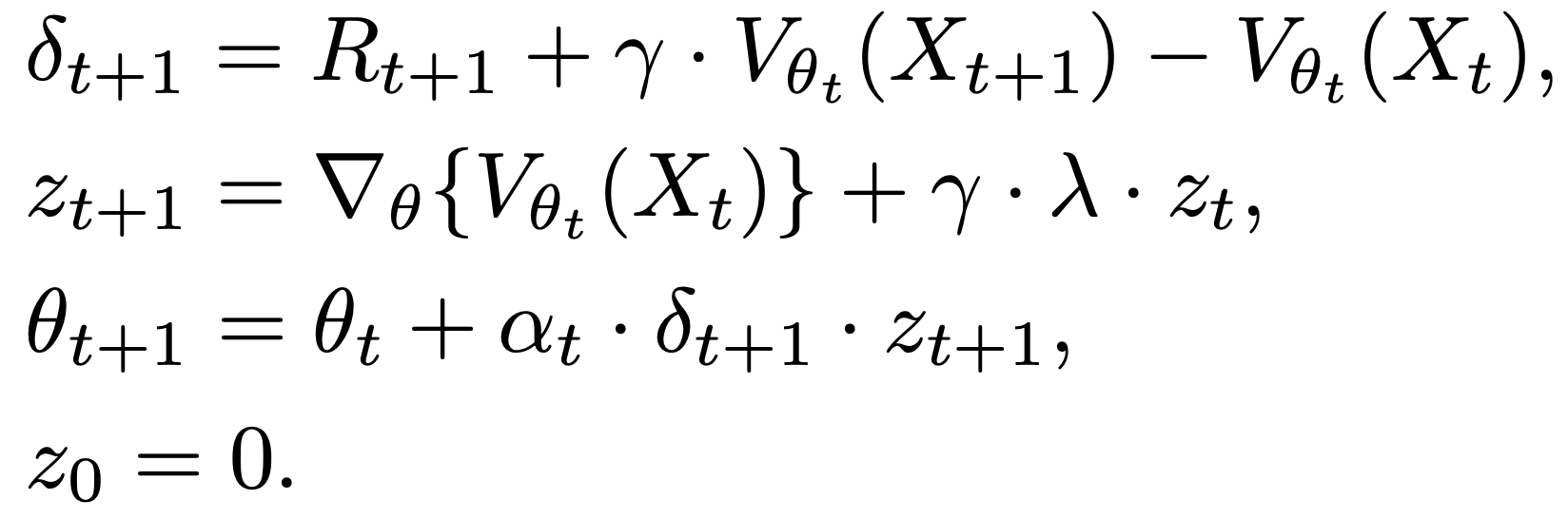
Where $\delta$ is the error of the function approximator, $V_{\theta}$ is the value function approximator with $\theta$ as its parameters. $\gamma$ is the discount rate, and $\alpha$ is the learning rate. $X$ is the feature representaion of (a) state. $z$ is the elibility traces.
Note how the idea of the elibility traces resembles the idea of the momentum in the optimization methods.
A review of the environment
A car is on a one-dimensional track, positioned between two “mountains”. The goal is to drive up the mountain on the right; however, the car’s engine is not strong enough to scale the mountain in a single pass. Therefore, the only way to succeed is to drive back and forth to build up momentum.
The car’s state, at any point in time, is given by a two-dimensional vector containing its horizonal position and velocity. The car commences each episode stationary, at the bottom of the valley between the hills (at position approximately -0.5), and the episode ends when either the car reaches the flag (position > 0.5).
At each move, the car has three actions available to it: push left, push right or do nothing, and a penalty of 1 unit is applied for each move taken (including doing nothing). This actually allows for using the exploration technique called optimistic initial values.
Results
After training the model, the results are shown as the follows:
The performance of the optimal policy:
We also record (a video for) the performance of the algorithm for the optimal policy.
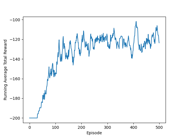
Average total reward over different episodes:
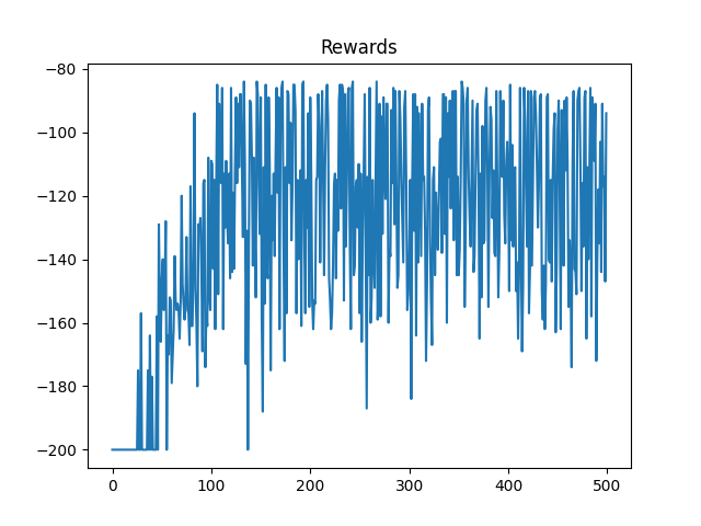
As you can see it is very volatile. It is better to take a look at the running average of this figure, which is practically at each point, it is the average of the 10 recent steps. It reduces the effect of the randomness of the initial point, and helps us with interpreting the results.
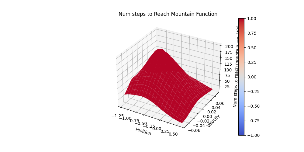
And the average # steps to reach to the top of the mountain at different state-action pairs (which is practically $(-Q^*(s,a))$) is shown in the following figure:
To see the Github repository for this project, see Github.