
Policy Gradient with Baseline in Continuous Action Space
Published:
As we know, polciy gradient approaches aim at directly modeling the policy and trying to optimize it. When the number of actions are limited, we can model the probabilities for each of the many actions separately, and sample an action using those probabilities. An example of such problems is this project.
However, this approach is not available when we have continuous action space. The strategy that we can take in thise cases is to assume that the optimal policy is a (Gaussian) probaility distribution function, and when making a decision we sample from this distribution. The task then becomes to learn the parameters of this probability distribution (in this case: mean and covariance matrix).
We also use baseline to decrease the variance of the model. A good choice for the baseline is to use the state value functions, V(s), which means that we need a value function approximator to estimate V(s) as well.
Now, assume that the neural network that we use for estimating the parameters of the probability distribution function of the policy (i.e. the policy model) has the parameter θ that we need to estimate, and the neural network that we use for estimating the value function V(s) has the parameters w. Now, the update rule for this algorithm is as follows: (See [1])
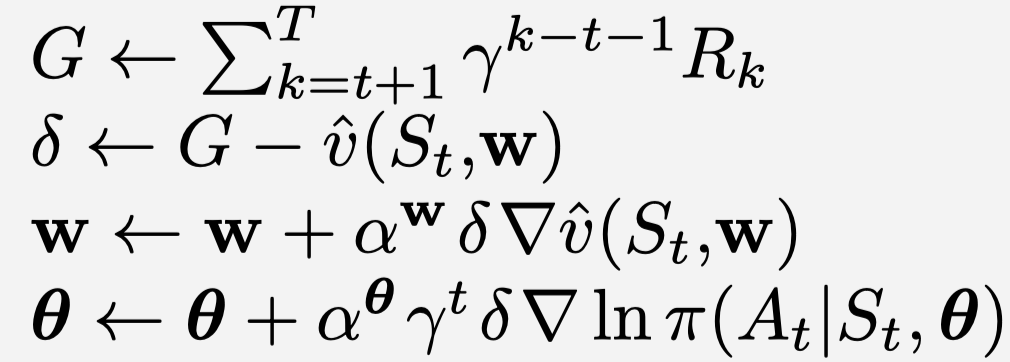
Now, since the Gaussian probability distribution function has two parameters, i.e. mean and std (recall that action is 1D), then we use two neural networks for the policy model, one estimating the mean and another estimates the std. The way we implement this is that we use the same set of hidden layers and just connect two different output layers: one (output) layer defines the neural netowrk for finding the mean, and the other (output) layer defines the other neural network used for finding the std.
An implementation chanllebge is: How to manually calculate the gradient? We need the gradient to train the policy models. This is an iplementaiton challenge, rather than a theoretical one. If, for instance, we use neural networks as the function approximator, then calculating the gradient of the objective funciton w.r.t. the weights could be troublesome. There is an interesting trick that we can use to do this. We can use the automatic differentiation provided in Tensorflow. The trick is to use only operations that keras “knows about” aka that exist as operations in TensorFlow, and the TensorFlow will automatically a graph of operations to backpropagate against. Now, in order to do this, we manually implement a hidden layer in the code, and the fully connected neural network that we are using for the policy gradient is created by adding one layer after another. This allows TensorFlow to do automatic differentiation.
The Environment:
The problem that we apply this method is the MountainCarContinuous-v0 which has only one action: The amount of the force that the car is pushed, which is continuous. The goal is to drive up the mountain on the right; however, the car’s engine is not strong enough to scale the mountain in a single pass. The car’s state, at any point in time, is given by a two-dimensional vector containing its horizonal position and velocity. The car commences each episode stationary, at the bottom of the valley between the hills (at position approximately -0.5), and the episode ends when either the car reaches the flag (position > 0.5).
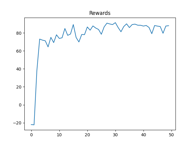
Results
We apply this method to the Cart Pole environment. The results is shown in the following figure:
We also record (a video for) the performance of the algorithm for the optimal policy.
To see the Github repository for this project, see Github.